


1 Introduction
Energy disaggregation, also known as non-intrusive load monitoring (NILM), is the task of separating aggregate energy data for a whole building into the energy data for individual appliances[1]. It can help users in optimizing energy consumption behaviors and identifying behavioral trends. It’s beneficial to utility companies to strategically market products to consumers; to electricity grid planners to predict grid loads; to appliance manufactures to improve control[2]. Prior studies indicate that building electricity consumption can be reduced by up to 10 to 15% using better energy management[3].
Many energy disaggregation techniques have been proposed to model appliance operation, extract electrical features, and perform classification[2]. Supervised machine learning have been applied to perform classification and optimization to design classifiers such as Naive Bayes, k-means, neural networks (NN), support vector machine (SVM), Hidden Markov Model, and many hybrid approaches[2,4-5], but they rely on medium or high frequency monitoring data and parameter adjust algorithm. In real world scenarios, this assumption not only request expensive high-sampling frequency sensors and sensitivity to the noise of other appliances, but also the increased cost of computational time and storage with large scale of smart metering deployment on the way[6,7]. In recent decades, Paradiso F[8]implement a multilayer perceptron NN with back propagation algorithm to classify the low-frequency monitoring data. This method is prone to converge to a local minimum and high computational cost. the low-frequency monitoring data is 1 sample each one minutes (or more longer time) gathered by meters (i. e. smart plugs) distributed in the home[8,9]. Liao J[9]proposed a low-complexity supervised approach decision trees method on NILM with sampling rates in the order of seconds and minutes, using active power measurements. Altrabalsi H[10]develop an alternative approach based on SVM and k-means, where k-means is used to reduce the SVM training set size by identifying only the representative subset of the original dataset for the SVM training. However, the quality of SVM models depends on a proper setting of SVM meta-parameters, tuning several SVM parameters is very expensive in terms of computational costs and data requirements[11]. The SVM models are not suitable for real-time NILM application, either due to modest performance or high execution time.
This paper proposes a multi-output extreme learning machine (MO-ELM) based energy disaggregation for low-frequency monitoring data gathered by meters distributed in the home without any priori knowledge concerning special appliances to set initial model. The new proposed learning algorithm can be easily implemented, reach the smallest training error, obtain the smallest norm of weights and good generalization performance, and run extremely fast.
The remainder of this paper is organized as follows. In Section 2, briefly reviews ELM methods. In Section 3, MO-ELM based energy disaggregation is proposed. Experimental results are reported in Section 4, and finally presents the research findings and future expectation and planning in Section 5.
2 Multi-output Extreme Learning Machine
This section will introduce the basic knowledge related to MO-ELM classifiers, so as to facilitate the description of subsequent system design and basic introduction of the personnel with irrelevant background. The ELM algorithm was originally proposed by Huang for single-hidden layer feed-forward neural networks (SLFNs)[12].
Given a training dataset, T = {(xi, ti)|xi ∈Rn, ti ∈Rm, i = 1, 2,…,N}, where xi is a n×1 input vector and ti is a m×1 target vector, the output of ELM is
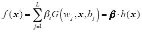
where, wj = [wj1,wj2,…,wjL]T and βj = [βj1, βj2, …,βjL]T are the weight vector connecting the j th hidden node with the input nodes and the output nodes, respectively, G(wj,x,bj) is the output of the j th hidden node and h(x) = [G(w1,x,b1), …,G(wL,x,bL)]T is the output vector of the hidden layer with respect to the input x, h(x) actually maps the data from the d-dimensional input space to the L-dimensional hidden layer feature space H. In Ref.[13] it is proved that the hidden layer weights and biases are randomly chosen and the output weights are analytically determined by finding the least-square solution in a SLFN. The NN is obtained after a few steps with very low computational cost and extremely fast learning speed. In Ref.[14-15] ELM was extended to the "generalized" SLFNs which may not be neuron alike.
For the binary classification applications, the decision function of ELM is
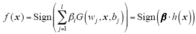
Different from traditional learning algorithms for NN, ELM not only tends to reach the smallest training error but also the smallest norm of output weights. Bartlett’s theory[16] shows that for feed forward NN reaching smaller training error, the smaller the norm of weights is, the better generalization performance the networks tend to have. We conjecture that this error as well as the norm of the output weights
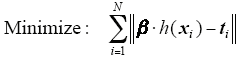
Multi-class applications is to let ELM have multi-output nodes instead of a single-output node. m-class classifiers have m output nodes. If the original class label is p, the expected output vector of the m output nodes is 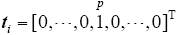
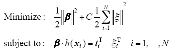
where ξi = [ξi ,1,…,ξi ,m]T is the training error vector of the output nodes with respect to the training sample xi. Based on the KKT theorem, to train ELM is equivalent to solving one convex optimization problem.
the output function of multi-output ELM classifier is
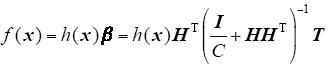
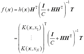
If a feature mapping h(x) is unknown to users, one can apply Mercer’s conditions on ELM. We can define a kernel matrix for ELM as follows

Then, the output function of ELM classifier Equ.(5) can be written compactly as
According to ELM theories[11,12,13,14,15,16], the ELM have less optimization constraints and better generalization performance than SVM. and the paper[17] also pointed out that the generalization performance of ELM is less sensitive to the learning parameters especially the number of hidden nodes. Thus, compared to SVM, users can use ELM easily and effectively by avoiding tedious and time-consuming parameter tuning.
3 Energy Disaggregation Based on MO-ELM
In this section, the paper describe the proposed energy disaggregation method based on MO-ELM. Due to the low energy monitoring sampling rate, only the load series of the active power consumption with time resolution down to 1s is analyzed. The focus of the proposed methods is on steady state information. In the following, we describe the whole procedure.
Let’s consider p(ti) the measured active power at time ti, which is the output of pre-processing module in energy disaggregation procedure. We denote as p(ti) = p(iT) = p(i) where T = ti - ti-1 is the sampling interval.
The disaggregation task is to find pj(i) for all j appliances in a set of all known household’s appliances, such that 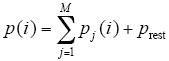
The entire disaggregation procedure includes four steps: data-pre-processing, event detection, feature extraction, a training and classification.
3.1 Data Pre-Processing
After the raw power data are captured from sub-meter, the pre-processing is responsible for identifying corrupted data and amending the faulty data, according to the error type[18]. It includes data normalization for standardization purpose and compe- nsation for certain power-quality-related issues[19].
3.2 Event Detection
State changes of one or more appliance in the time-series aggregate load curve are detected and handled by events detection. These events contain the information about all involved electric appliances. It is neither efficient nor practical in the pre-processing step to store and process all data, so our load disaggregation procedure will detect when there is an actual appliance being switched (on/off). In our case, we use an effective edge detection method of [8-9,20] and focus on improving the feature extraction and classification steps.
Appliance state change detection is implemented by comparing |pj(i) - pj(i - 1)| with W, where W is a threshold. If |pj(i) - pj(i - 1)|≥W, we say that the appliance j has changed state at time instant iT. Threshold W depends on the appliance set M and must be set low enough so that for all j, if |pj(i) - pj(i - 1)|≤W, appliance j did not change its state and, otherwise, it did. All appliances that operate below threshold W will not be detected. W is set based on the minimum state transition that needs to be detected and the maximum variation of the active power within one appliance state across all appliances’ states; that is
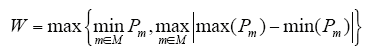
where Pm is a vector of readings of appliance m.
When an event occurs whenever an appliance changes its state, edge detection is used to detect events by comparing |pj(i) - pj(i - 1)| with W. We say a window of the event started at time ls and ended at le if an appliance changes its state at ls and le, and
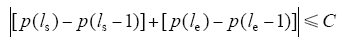
where C is a parameter, that is estimated in practice heuristically based on the detected rising edge. The higher the rising edge (device with high power consumption), the lower the value of C, e.g., C for electrical shower is 5% and for refrigerator is 25%.
The appliance event window include appliance consumption details.
3.3 Feature Extraction
The feature extraction block process the detected event provided by the event detection step to build a vector of feature and stored, the extract feature include the distinguishing characteristics of the aggregate load curve.
Extracted features could be simply all active power readings in the event window, including the first increasing edge at the start of the event and the last decreasing edge at the end of the event, that is, |[p(ls) - p(ls - 1)]| = Δp(ls) and |[p(le) - p(le - 1)]| = Δp(le), maximum/minimum value, the mean value for active power, the standard deviation of active power value, the RMS of active power value. This study designed a data structure to store power features, as shown in Table 1. We will then submit these features to extreme learning machine algorithms to perform disaggregation.
Tab.1 Data structure of feature parameters
| Data type | Function | Description |
|---|---|---|
| Float | F-inc | the first increasing edge value Δp(ls) |
| Float | L-dec | the last decreasing edge value Δp(le) |
| Float | Max | the maximum active power value in the event window |
| Float | Min | the minimum active power value in the event window |
| Float | Avg | the mean active power value in the event window |
| Float | med | the median active power value in the event window |
| Float | Std_dev | the standard deviation active power value in the event window |
| Float | Rms | the RMS active power value in the event window |
3.4 Training & Classification
Energy disaggregation with supervised machine learning for a household comprises two phases: training phase and testing phase. In training phase, the algorithm build the MO-ELM classification model with all stored event features which are examined along with the logs, that shows which appliances triggered the event. Once the multi-output ELM classification model is built, the model is ready to classify the extracted features from detected event of a household aggregated power consumption in testing phase.
The formulation process is as follows, xi∈Rn, i = 1,2,…,N is comprised of appliance features as plugged in socket and switched on, ti∈Rm, i = 1,2,…,N correspond to m appliance. The ELM model Equ.(4) is built by using multi-output ELM classifier.
when the appliance state changes have been identified and the feature xtest extracted for the aggregate load in the household without the labeled, energy disaggregation for a household aggregated power consumption using the ELM method is straightforward. In comparison to other energy disaggregation techniques, the ELM method will run more quickly and can solve the output f(xtest) at one time. The output model f(xtest) is the appliance energy state.
As will be shown in the next section, the trained ELM model is relatively quicker than SVM based model.
4 Real Household Experiment and Result Analysis
4.1 Data Description of Energy Disaggregation in House
In order to evaluate the performance of the multi-output ELM algorithm for energy disaggregation, the actual electricity consumption measurements released by Kolteret al[21] at http://redd.csail.mit.edu. are used here. All households' appliances for which individual power consumption was not available, were considered unknown and hence they contribute to noise prest. The dataset contains both appliance and total consumption level data from six households in the USA collected in April and May 2011. Some of the houses contain a single appliance (e.g., a dishwasher), other houses contain multiple appliances (e.g., lights, kitchen outlets), there are approximately 20 consecutive days of measurements available for each house.
4.2 Experiments and Result Analysis
In this study, we chose the representative energy consuming appliances in houses #1 and houses #2, 4 appliances from the 20 multiple appliances in houses #1 and 4 appliances from the 11 multiple appliances in houses #2 (general information about experiments datasets is briefly introduced in Table 2). All consumption level data is sampled at a low sampling rates (1min) from the low frequency power data (1Hz) of the REDD.
Tab.2 Information of the chosen appliances of house # 1 and # 2 in REDD
| Houses no. | Variable no. | Used variables | Houses no. | Variable no. | Used variables | |
|---|---|---|---|---|---|---|
| house # 1 | 3 | oven | house # 2 | 5 | stove | |
| 5 | refrigerator | 6 | microwave | |||
| 6 | dishwasher | 9 | refrigerator | |||
| 11 | microwave | 10 | dishwasher |
Here we present an experiment to compare the performance of SVM disaggregation method with the proposed MO-ELM approach with REDD.
The raw data are captured from sub-meter, we extracted two week of data by selecting four types of appliances after event detecting and extracted feature is used for training. i.e.60% of the total dataset collected using submetering at a circuit level including just a single appliance in house #1 and house #2 respectively for training. The rest data of one week is used for testing. i.e.40% of the total dataset for testing. All the features have been normalized into [1, -1].
Testing has been performed using Matlab version R2012a on a machine equipped with an intel Core(TM) I7-4770k at 3.5GHz, 8.0GB RAM. The (Gaussian) radial basis function kernel is a popular kernel function used in support vector regression. It is defined as
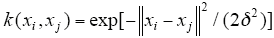
Experiments are conducted using the LIBSVM[22] to solve the SVC model, in order to typically evaluate the performance difference of classifier models, they have the same kernel parameters.
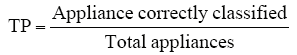
One type of rate is used: namely the fraction true-positive (TP). The TP defined in Equ. (11) is computed as the fraction of the number of correctly classified appliance samples to the total number of appliance.
The experiment results are shown in Table 3.
Tab.3 Disaggregation results for submetered data
| Houses no. | Train time/s | Performance comparison the rate of change | Test time/s | Performance comparison the rate of change | TP | Performance comparison the rate of change | |||
|---|---|---|---|---|---|---|---|---|---|
| SVM | ELM | SVM | ELM | SVM | ELM | ||||
| House1 | 0.058 | 0.040 | ↓31.03% | 0.034 | 0.017 | ↓50.00% | 0.9188 | 0.9440 | ↑ 2.74% |
| House2 | 0.891 | 0.221 | ↓75.19% | 0.187 | 0.065 | ↓65.24% | 0.9095 | 0.9129 | ↑3.74% |
Table 3 shows the classification results for four appliances. It can be seen from Table 3 that the MO-ELM approach always outperforms the SVM-based method, it requires less time for both training and testing, and with the same time have higher TP; decrease the train time from 0.058 s to 0.040 s and from 0. 891 s to 0.221 s, decrease the test time from 0.034 s to 0.017 s and from 0.187 s to 0.065 s, increase the TP from 91.88% to 94.40% and from 90.95% to 91.29%.
5 Conclusion and Future Work
In this paper, we have proposed an approach for energy disaggregation by exploiting low-frequency measurement data based on the MO-ELM. The presented results clearly demonstrate that energy disaggregation using MO-ELM can obtain a fairly less train and test time than SVM, at the same time improve the performance indicators significantly.
In the future, we would use the MO-ELM to study energy, energy consumption patterns and sustainability problems in different frequency dataset.
参考文献
Nonintrusive appliance load monitoring
[J].
DOI:10.3390/s19163621
URL
PMID:31434283
[本文引用: 1]

Nonintrusive appliance load monitoring (NIALM) allows disaggregation of total electricity consumption into particular appliances in domestic or industrial environments. NIALM systems operation is based on processing of electrical signals acquired at one point of a monitored area. The main objective of this paper was to present the state-of-the-art in NIALM technologies for the smart home. This paper focuses on sensors and measurement methods. Different intelligent algorithms for processing signals have been presented. Identification accuracy for an actual set of appliances has been compared. This article depicts the architecture of a unique NIALM laboratory, presented in detail. Results of developed NIALM methods exploiting different measurement data are discussed and compared to known methods. New directions of NIALM research are proposed.
Nonintrusive appliance load monitoring: review and outlook
[J].Consumer systems for home energy management can provide significant energy saving. Such systems may be based on nonintrusive appliance load monitoring (NIALM), in which individual appliance power consumption information is disaggregated from single-point measurements. The disaggregation methods constitute the most important part of NIALM systems. This paper reviews the methodology of consumer systems for NIALM in residential buildings.(1)
Advanced metering initiatives and residential feedback programs: a meta-review for household electricity-saving opportunities
[C].
NILM redux: the case for emphasizing applications over accuracy[R]. NILM-2014 Workshop, Austin,
Genetic algorithm for pattern detection in NIALM systems
[C].
A low-complexity energy disaggregation method: performance and robustness
[C].
ANN-based appliance recognition from low-frequency energy monitoring data
[C].
Non-intrusive appliance load monitoring using low-resolution smart meter data
[C].
A low-complexity energy disaggregation method: performance and robustness
[C].
Support vector machine applications in the field of hydrology: a review
[J].DOI:10.1016/j.asoc.2014.02.002 URL [本文引用: 2]
Extreme learning machine: theory and applications
[J].
DOI:10.1063/1.5123013
URL
PMID:31757143
[本文引用: 2]
The study of matter at extreme densities and temperatures as they occur in astrophysical objects and state-of-the-art experiments with high-intensity lasers is of high current interest for many applications. While no overarching theory for this regime exists, accurate data for the density response of correlated electrons to an external perturbation are of paramount importance. In this context, the key quantity is given by the local field correction (LFC), which provides a wave-vector resolved description of exchange-correlation effects. In this work, we present extensive new path integral Monte Carlo (PIMC) results for the static LFC of the uniform electron gas, which are subsequently used to train a fully connected deep neural network. This allows us to present a representation of the LFC with respect to continuous wave-vectors, densities, and temperatures covering the entire warm dense matter regime. Both the PIMC data and neural-net results are available online. Moreover, we expect the presented combination of ab initio calculations with machine-learning methods to be a promising strategy for many applications.
Universal approximation using incremental constructive feed forward networks with random hidden nodes
[J].
DOI:10.1109/TNN.2006.875977
URL
PMID:16856652
[本文引用: 1]
According to conventional neural network theories, single-hidden-layer feedforward networks (SLFNs) with additive or radial basis function (RBF) hidden nodes are universal approximators when all the parameters of the networks are allowed adjustable. However, as observed in most neural network implementations, tuning all the parameters of the networks may cause learning complicated and inefficient, and it may be difficult to train networks with nondifferential activation functions such as threshold networks. Unlike conventional neural network theories, this paper proves in an incremental constructive method that in order to let SLFNs work as universal approximators, one may simply randomly choose hidden nodes and then only need to adjust the output weights linking the hidden layer and the output layer. In such SLFNs implementations, the activation functions for additive nodes can be any bounded nonconstant piecewise continuous functions g : R --> R and the activation functions for RBF nodes can be any integrable piecewise continuous functions g : R --> R and integral of R g(x)dx not equal to 0. The proposed incremental method is efficient not only for SFLNs with continuous (including nondifferentiable) activation functions but also for SLFNs with piecewise continuous (such as threshold) activation functions. Compared to other popular methods such a new network is fully automatic and users need not intervene the learning process by manually tuning control parameters.
Convex incremental extreme learning machine
[J].
DOI:10.1109/TCYB.2018.2830338
URL
PMID:29994325
[本文引用: 1]
Fault diagnosis is important to the industrial process. This paper proposes an orthogonal incremental extreme learning machine based on driving amount (DAOI-ELM) for recognizing the faults of the Tennessee-Eastman process (TEP). The basic idea of DAOI-ELM is to incorporate the Gram-Schmidt orthogonalization method and driving amount into an incremental extreme learning machine (I-ELM). The case study for the 2-D nonlinear function and regression problems from the UCI dataset results show that DAOI-ELM can obtain better generalization ability and a more compact structure of ELM than I-ELM, convex I-ELM (CI-ELM), orthogonal I-ELM (OI-ELM), and bidirectional ELM. The experimental training and testing data are derived from the simulations of TEP. The performance of DAOI-ELM is evaluated and compared with that of the back propagation neural network, support vector machine, I-ELM, CI-ELM, and OI-ELM. The simulation results show that DAOI-ELM diagnoses the TEP faults better than other methods.
Enhanced random search based incremental extreme learning machine
[J].DOI:10.1016/j.neucom.2007.10.008 URL [本文引用: 1]
The sample complexity of pattern classification with neural networks: the size of the weights is more important than the size of the network
[J].DOI:10.1109/18.661502 URL [本文引用: 2]
Optimization method based extreme learning machine for classification
[J].
DOI:10.1186/s12859-019-3228-0
URL
PMID:31888444
[本文引用: 1]
The main goal of successful gene selection for microarray data is to find compact and predictive gene subsets which could improve the accuracy. Though a large pool of available methods exists, selecting the optimal gene subset for accurate classification is still very challenging for the diagnosis and treatment of cancer.
Power system quality assessment
[M].
Power disaggregation for low-sampling rate data
[C].
Disaggregation of home energy display data using probabilistic approach
[J].Home energy displays are emerging home energy management devices. Their energy saving potential is limited, because most display whole-home electricity consumption data. We propose a new approach to disaggregation electricity consumption by individual appliances and/or end uses that would enhance the effectiveness of home energy displays. The proposed method decomposes a system of appliance models into tuplets of appliances overlapping in power draw. Each tuplet is disaggregated using a modified Viterbi algorithm. In this way, the complexity of the disaggregation algorithm is linearly proportional to the number of appliances. The superior accuracy of the method is illustrated by a simulation example and by actual household data(1).
LIBSVM: a library for support vector machines
[J].
DOI:10.3389/fpsyt.2019.00585
URL
PMID:31474890
[本文引用: 1]
The nucleus accumbens (NAc) plays an important role in the reward circuit, and abnormal regional activities of the reward circuit have been reported in various psychiatric disorders including somatization disorder (SD). However, few researches are designed to analyze the NAc connectivity in SD. This study was designed to explore the NAc connectivity in first-episode, drug-naive patients with SD using the bilateral NAc as seeds. Twenty-five first-episode, drug-naive patients with SD and 28 healthy controls were recruited. Functional connectivity (FC) was designed to analyze the images. LIBSVM (a library for support vector machines) was used to identify whether abnormal FC could be utilized to discriminate the patients from the controls. The patients showed significantly increased FC between the left NAc and the right gyrus rectus and left medial prefrontal cortex/anterior cingulate cortex (MPFC/ACC), and between the right NAc and the left gyrus rectus and left MPFC/ACC compared with the controls. The patients could be separated from the controls through increased FC between the left NAc and the right gyrus rectus with a sensitivity of 88.00% and a specificity of 82.14%. The findings reveal that patients with SD have increased NAc connectivity with the frontal regions of the reward circuit. Increased left NAc-right gyrus rectus connectivity can be used as a potential marker to discriminate patients with SD from healthy controls. The study thus highlights the importance of the reward circuit in the neuropathology of SD.
